Artificial intelligence (AI) in healthcare is predominantly built on observational data that provide incomplete, delayed, and noisy representations of underlying biological processes. Such limitations constrain current predictive models, which often remain reactive and fail to capture the intrinsic dynamics of disease evolution. In this study, we introduce a novel AI-driven framework based on latent-state reconstruction, designed to infer hidden disease trajectories from partial clinical and population-level observations and to generate dynamic, forward-looking risk estimates. The proposed approach departs fundamentally from traditional methods by explicitly modeling healthcare systems as partially observed complex adaptive systems. It reconstructs latent health states that evolve over time and gives rise to observable clinical measurements subject to stochastic variability. Drawing a conceptual parallel to quantum mechanics, where a system’s true state is described by a wave function that governs probabilistic observations, our framework treats the latent health state as the primary object of inference rather than the observed data alone. This shift enables a transition from descriptive analytics to anticipatory intelligence. By deriving hazard functions from reconstructed latent trajectories, the framework provides earlier and more accurate detection of disease progression, outbreak dynamics, and systemic instability. Empirical and theoretical analysis demonstrates that this approach captures underlying population heterogeneity and temporal dynamics that are inaccessible to conventional models. This work establishes a new paradigm for AI in healthcare, where prediction is grounded in the reconstruction of hidden system dynamics, enabling proactive intervention and more reliable decision-making in complex, high-dimensional environments.
| Published in | Journal of Family Medicine and Health Care (Volume 12, Issue 1) |
| DOI | 10.11648/j.jfmhc.20261201.11 |
| Page(s) | 1-13 |
| Creative Commons |
This is an Open Access article, distributed under the terms of the Creative Commons Attribution 4.0 International License (http://creativecommons.org/licenses/by/4.0/), which permits unrestricted use, distribution and reproduction in any medium or format, provided the original work is properly cited. |
| Copyright |
Copyright © The Author(s), 2026. Published by Science Publishing Group |
Latent-state Reconstruction, Artificial Intelligence in Healthcare, Predictive Analytics, Hazard Function, Complex Adaptive Systems, Disease Progression Modeling, Early Detection
Variable | Meaning |
|---|---|
| Age, |
| Blood pressure |
| Treatment indicator |
| Biomarker level |
AI | Artificial Intelligence |
LAT-AI | Latent Adaptive Transformative AI |
SAIHA | Stochastic Augmented Integrated Hazard Analysis |
| [1] | Kaplan EL, Meier P. Nonparametric estimation from incomplete observations. J Am Stat Assoc. 1958; 53(282): 457–481. |
| [2] | de Melo P. Public Health Informatics and Technology. Washington, DC: Library of Congress; 2024. |
| [3] | Seifert J, Shao Y, Mosk AP. Noise-robust latent vector reconstruction in ptychography using deep generative models. Opt Express. 2024; 32(1): 1020–1033. |
| [4] | Singh A, Ogunfunmi T. An overview of variational autoencoders for source separation, finance, and bio-signal applications. Entropy (Basel). 2022; 24(1): 55. |
| [5] | Yu S, Príncipe JC. Understanding autoencoders with information theoretic concepts. Neural Netw. 2019; 117: 104–123. |
| [6] | Kingma DP, Welling M. An introduction to variational autoencoders. Found Trends Mach Learn. 2019; 12: 307–392. |
| [7] | Asperti A, Trentin M. Balancing reconstruction error and Kullback–Leibler divergence in variational autoencoders. IEEE Access. 2020; 8: 199440–199448. |
| [8] | Blei DM, Kucukelbir A, McAuliffe JD. Variational inference: a review for statisticians. J Am Stat Assoc. 2017; 112: 859–877. |
| [9] | Seki S, Kameoka H, Li L, Toda T, Takeda K. Underdetermined source separation based on generalized multichannel variational autoencoder. IEEE Access. 2019; 7: 168104–168115. |
| [10] | Schober P, Vetter TR. Survival analysis and interpretation of time-to-event data: the tortoise and the hare. Anesth Analg. 2018; 127(3): 792–798. |
| [11] | Pang M, Platt RW, Schuster T, Abrahamowicz M. Spline-based accelerated failure time model. Stat Med. 2021; 40(2): 481–497. |
| [12] | Arcuri LJ, Souza Santos FP, Perini GF, Hamerschlak N. Fine and Gray or Cox model? Blood Adv. 2024; 8(6): 1420–1421. |
| [13] | de Melo P, DiLella M, Holman T, McElveen S. Accurate prediction of survival based on Kaplan–Meier analytics. Cancer Res J. 2025; 13(4). |
| [14] | Cox DR. The regression analysis of binary sequences. J R Stat Soc Series B. 1958; 20: 215–232. |
| [15] | Silva DG, Fantinato DG, Canuto JC, Duarte LT, Neves A, Suyama R, Montalvão J, de Faissol Attux R. An introduction to information theoretic learning, Part I: foundations. J Commun Inf Syst. 2016; 31. |
| [16] | Williams RJ. Simple statistical gradient-following algorithms for connectionist reinforcement learning. Mach Learn. 1992; 8: 229–256. |
| [17] | Gao R, Hou X, Qin J, Chen J, Liu L, Zhu F, Zhang Z, Shao L. Zero-VAE-GAN: generating unseen features for generalized and transductive zero-shot learning. IEEE Trans Image Process. 2020; 29: 3665–3680. |
APA Style
Melo, P. D. (2026). Anticipatory Healthcare Analytics: Inferring Latent Disease Dynamics from Noisy Clinical Observations. Journal of Family Medicine and Health Care, 12(1), 1-13. https://doi.org/10.11648/j.jfmhc.20261201.11
ACS Style
Melo, P. D. Anticipatory Healthcare Analytics: Inferring Latent Disease Dynamics from Noisy Clinical Observations. J. Fam. Med. Health Care 2026, 12(1), 1-13. doi: 10.11648/j.jfmhc.20261201.11
@article{10.11648/j.jfmhc.20261201.11,
  author = {Philip de Melo},
  title = {Anticipatory Healthcare Analytics: Inferring Latent Disease Dynamics from Noisy Clinical Observations},
  journal = {Journal of Family Medicine and Health Care},
  volume = {12},
  number = {1},
  pages = {1-13},
  doi = {10.11648/j.jfmhc.20261201.11},
  url = {https://doi.org/10.11648/j.jfmhc.20261201.11},
  eprint = {https://article.sciencepublishinggroup.com/pdf/10.11648.j.jfmhc.20261201.11},
  abstract = {Artificial intelligence (AI) in healthcare is predominantly built on observational data that provide incomplete, delayed, and noisy representations of underlying biological processes. Such limitations constrain current predictive models, which often remain reactive and fail to capture the intrinsic dynamics of disease evolution. In this study, we introduce a novel AI-driven framework based on latent-state reconstruction, designed to infer hidden disease trajectories from partial clinical and population-level observations and to generate dynamic, forward-looking risk estimates. The proposed approach departs fundamentally from traditional methods by explicitly modeling healthcare systems as partially observed complex adaptive systems. It reconstructs latent health states that evolve over time and gives rise to observable clinical measurements subject to stochastic variability. Drawing a conceptual parallel to quantum mechanics, where a system’s true state is described by a wave function that governs probabilistic observations, our framework treats the latent health state as the primary object of inference rather than the observed data alone. This shift enables a transition from descriptive analytics to anticipatory intelligence. By deriving hazard functions from reconstructed latent trajectories, the framework provides earlier and more accurate detection of disease progression, outbreak dynamics, and systemic instability. Empirical and theoretical analysis demonstrates that this approach captures underlying population heterogeneity and temporal dynamics that are inaccessible to conventional models. This work establishes a new paradigm for AI in healthcare, where prediction is grounded in the reconstruction of hidden system dynamics, enabling proactive intervention and more reliable decision-making in complex, high-dimensional environments.},
 year = {2026}
}
TY  - JOUR
T1  - Anticipatory Healthcare Analytics: Inferring Latent Disease Dynamics from Noisy Clinical Observations
AU  - Philip de Melo
Y1  - 2026/04/28
PY  - 2026
N1  - https://doi.org/10.11648/j.jfmhc.20261201.11
DO  - 10.11648/j.jfmhc.20261201.11
T2  - Journal of Family Medicine and Health Care
JF  - Journal of Family Medicine and Health Care
JO  - Journal of Family Medicine and Health Care
SP  - 1
EP  - 13
PB  - Science Publishing Group
SN  - 2469-8342
UR  - https://doi.org/10.11648/j.jfmhc.20261201.11
AB  - Artificial intelligence (AI) in healthcare is predominantly built on observational data that provide incomplete, delayed, and noisy representations of underlying biological processes. Such limitations constrain current predictive models, which often remain reactive and fail to capture the intrinsic dynamics of disease evolution. In this study, we introduce a novel AI-driven framework based on latent-state reconstruction, designed to infer hidden disease trajectories from partial clinical and population-level observations and to generate dynamic, forward-looking risk estimates. The proposed approach departs fundamentally from traditional methods by explicitly modeling healthcare systems as partially observed complex adaptive systems. It reconstructs latent health states that evolve over time and gives rise to observable clinical measurements subject to stochastic variability. Drawing a conceptual parallel to quantum mechanics, where a system’s true state is described by a wave function that governs probabilistic observations, our framework treats the latent health state as the primary object of inference rather than the observed data alone. This shift enables a transition from descriptive analytics to anticipatory intelligence. By deriving hazard functions from reconstructed latent trajectories, the framework provides earlier and more accurate detection of disease progression, outbreak dynamics, and systemic instability. Empirical and theoretical analysis demonstrates that this approach captures underlying population heterogeneity and temporal dynamics that are inaccessible to conventional models. This work establishes a new paradigm for AI in healthcare, where prediction is grounded in the reconstruction of hidden system dynamics, enabling proactive intervention and more reliable decision-making in complex, high-dimensional environments.
VL  - 12
IS  - 1
ER  -
Nursing and Allied Health, Norfolk State University, Norfolk, United State
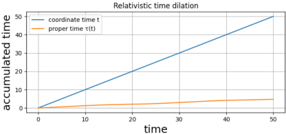
Figure 1. Comparison of coordinate time and relativistic proper time.
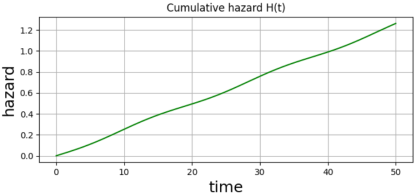
Figure 2. Cumulative hazard function .
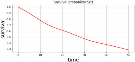
Figure 3. Survival probability .
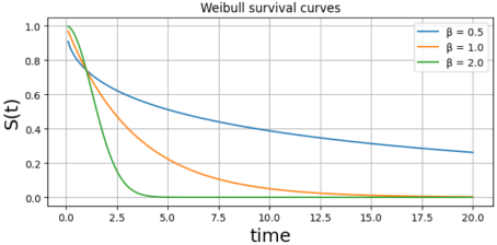
Figure 4. Weibull survival curves illustrating the effect of the shape parameter on survival dynamics.
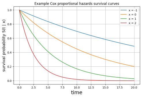
Figure 5. Cox proportional hazards survival curves.
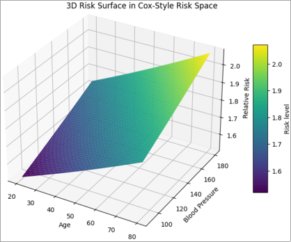
Figure 6. Three-dimensional risk surface in a Cox-style risk space defined by age and blood pressure, with glucose held constant.
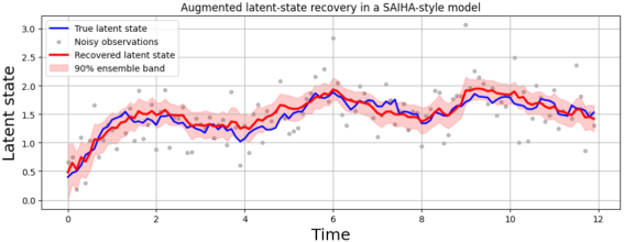
Figure 7. Recovery of a latent physiological state using the stochastic augmented integrated hazard analysis (SAIHA) framework.

Figure 8. Hazard functions derived from the latent health state in a SAIHA framework.
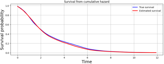
Figure 9. Survival probability derived from cumulative hazard in the SAIHA framework.
Information